# libraries
library(tidyverse)
library(sf)
library(spdep)

# theme
theme_set(theme_minimal())Working with PRIO-GRID data
Walkthrough of the PRIO-GRID data in R.
PRIO-GRID data
PRIO-GRID breaks up the Earth into a grid of little squares, or cells, each of which is 0.5 x 0.5 decimal degrees (roughly 50 x 50 km at the equator; you can read more about the data here). Researchers then conformed a variety of available spatial data to this grid system, giving users access to things like the population of each 50 x 50 km square everywhere on the globe.
The data come in three forms:
Shapefiles: information for plotting and doing spatial analysis on the grid systemStatic variables: data at the cell-level on stuff that doesn’t change (e.g., how mountainous that cell is)Yearly variables: data at the cell-level that changes over time (e.g., rain, population, etc.)
Spatial data in R
There are two main packages for dealing with spatial data in R:
spdep: older, richer set of functions, not-tidysf: newer, fewer functions, tidy
I would rather only use sf, but there are some nice functions in spdep we’ll need to use in this example that I’m not sure I can replicate in sf.
The starting point of the data is the cells themselves, stored as a shapefile. We can interact with shapefiles with the great sf library:
grid = read_sf("/Users/juan/Downloads/priogrid_cellshp/priogrid_cell.shp")
head(grid)
## Simple feature collection with 6 features and 5 fields
## Geometry type: POLYGON
## Dimension:     XY
## Bounding box:  xmin: 163.5 ymin: 89.5 xmax: 166.5 ymax: 90
## Geodetic CRS:  WGS 84
## # A tibble: 6 × 6
##      gid xcoord ycoord   col   row                                               geometry
##    <dbl>  <dbl>  <dbl> <dbl> <dbl>                                          <POLYGON [°]>
## 1 259168   164.   89.8   688   360 ((163.5 89.5, 163.5 90, 164 90, 164 89.5, 163.5 89.5))
## 2 259169   164.   89.8   689   360   ((164 89.5, 164 90, 164.5 90, 164.5 89.5, 164 89.5))
## 3 259170   165.   89.8   690   360 ((164.5 89.5, 164.5 90, 165 90, 165 89.5, 164.5 89.5))
## 4 259171   165.   89.8   691   360   ((165 89.5, 165 90, 165.5 90, 165.5 89.5, 165 89.5))
## 5 259172   166.   89.8   692   360 ((165.5 89.5, 165.5 90, 166 90, 166 89.5, 165.5 89.5))
## 6 259173   166.   89.8   693   360   ((166 89.5, 166 90, 166.5 90, 166.5 89.5, 166 89.5))
Each row in this tibble is a cell; there are almost 260,000 of them. The key columns are gid (a unique identifier for each grid cell) and geometry which {sf} can work with for map-making and other spatial data stuff.
Merging in the yearly data
The grid of cells itself doesn’t have much use without other information. We’ll need to merge in other variables, such as what country each cell is in. This is stored as yearly data by PRIO. Note: for the yearly variables we can choose a start and end date, but each variable varies in what years of data it has available. Below, I choose a few variables from the year 2010:
yearly_prio = read_csv("/Users/juan/Downloads/PRIO-GRID Yearly Variables for 2010-2010 - 2024-08-26.csv")
yearly_prio
## # A tibble: 64,818 × 9
##      gid  year agri_ih capdist  gwno nlights_mean pop_gpw_sum prec_gpcp  temp
##    <dbl> <dbl>   <dbl>   <dbl> <dbl>        <dbl>       <dbl>     <dbl> <dbl>
##  1 49182  2010      NA   2480.   155            0        9.68     1092. NA
##  2 49183  2010      NA   2483.   155            0       13.8      1092.  4.16
##  3 49184  2010      NA   2485.   155            0       43.6      1092.  4.50
##  4 49185  2010      NA   2488.   155            0        2.27     1092.  4.69
##  5 49186  2010       0   2492.   155            0        0        1324.  4.78
##  6 49898  2010      NA   2423.   155            0        1.71     1266.  3.84
##  7 49899  2010      NA   2422.   155            0       48.2      1266.  3.73
##  8 49900  2010      NA   2423.   155            0       43.7      1266.  3.61
##  9 49901  2010       0   2423.   155            0      132.       1092.  3.58
## 10 49902  2010       0   2425.   155            0      189.       1092.  3.70
## # ℹ 64,808 more rows
As you can see, I pulled nightlight data, population, precipitation, average temperatures, and the Gleditsch and Ward country identifiers (gwno).
We merge on gid:
grid_merged = left_join(grid, yearly_prio, by = "gid")
grid_merged |> head()
## Simple feature collection with 6 features and 13 fields
## Geometry type: POLYGON
## Dimension:     XY
## Bounding box:  xmin: 163.5 ymin: 89.5 xmax: 166.5 ymax: 90
## Geodetic CRS:  WGS 84
## # A tibble: 6 × 14
##      gid xcoord ycoord   col   row                                               geometry  year agri_ih capdist  gwno nlights_mean pop_gpw_sum prec_gpcp  temp
##    <dbl>  <dbl>  <dbl> <dbl> <dbl>                                          <POLYGON [°]> <dbl>   <dbl>   <dbl> <dbl>        <dbl>       <dbl>     <dbl> <dbl>
## 1 259168   164.   89.8   688   360 ((163.5 89.5, 163.5 90, 164 90, 164 89.5, 163.5 89.5))    NA      NA      NA    NA           NA          NA        NA    NA
## 2 259169   164.   89.8   689   360   ((164 89.5, 164 90, 164.5 90, 164.5 89.5, 164 89.5))    NA      NA      NA    NA           NA          NA        NA    NA
## 3 259170   165.   89.8   690   360 ((164.5 89.5, 164.5 90, 165 90, 165 89.5, 164.5 89.5))    NA      NA      NA    NA           NA          NA        NA    NA
## 4 259171   165.   89.8   691   360   ((165 89.5, 165 90, 165.5 90, 165.5 89.5, 165 89.5))    NA      NA      NA    NA           NA          NA        NA    NA
## 5 259172   166.   89.8   692   360 ((165.5 89.5, 165.5 90, 166 90, 166 89.5, 165.5 89.5))    NA      NA      NA    NA           NA          NA        NA    NA
## 6 259173   166.   89.8   693   360   ((166 89.5, 166 90, 166.5 90, 166.5 89.5, 166 89.5))    NA      NA      NA    NA           NA          NA        NA    NA
Cleaning the grid
We can take a couple more steps to make this data user-friendly. First, the Earth is mostly water so a lot of these cells are just water. We can get rid of the water by using the fact that the oceans (and other unclaimed territory) have missing gwno codes. Second, we can back out country names from gwno using {countrycodes}. Third, we can drop the coordinate variables:
clean_grid = grid_merged |>
  drop_na(gwno) |>
  mutate(country = countrycode::countrycode(gwno, origin = "gwn", destination = "country.name")) |>
  select(gid, year, country, geometry, capdist, nlights_mean, pop_gpw_sum, prec_gpcp, temp)

head(clean_grid)
## Simple feature collection with 6 features and 8 fields
## Geometry type: POLYGON
## Dimension:     XY
## Bounding box:  xmin: -76.5 ymin: 83 xmax: -73 ymax: 83.5
## Geodetic CRS:  WGS 84
## # A tibble: 6 × 9
##      gid  year country                                             geometry capdist nlights_mean pop_gpw_sum prec_gpcp  temp
##    <dbl> <dbl> <chr>                                          <POLYGON [°]>   <dbl>        <dbl>       <dbl>     <dbl> <dbl>
## 1 249328  2010 Canada  ((-76.5 83, -76.5 83.5, -76 83.5, -76 83, -76.5 83))   4216.           NA    0.00886       170. -20.3
## 2 249329  2010 Canada    ((-76 83, -76 83.5, -75.5 83.5, -75.5 83, -76 83))   4216.           NA    0.00612       170. -20.2
## 3 249330  2010 Canada  ((-75.5 83, -75.5 83.5, -75 83.5, -75 83, -75.5 83))   4216.           NA    0.000397      170. -20.2
## 4 249331  2010 Canada    ((-75 83, -75 83.5, -74.5 83.5, -74.5 83, -75 83))   4216.           NA    0.00357       172.  NA
## 5 249332  2010 Canada  ((-74.5 83, -74.5 83.5, -74 83.5, -74 83, -74.5 83))   4217.           NA    0.0119        172.  NA
## 6 249334  2010 Canada  ((-73.5 83, -73.5 83.5, -73 83.5, -73 83, -73.5 83))   4217.           NA    0.000209      172. -20.2
Notice that we are down to about 65,000 cells here. The oceans and Antartica are gone (and probably other stuff).
Plotting
The {sf} package works nicely with ggplot. We can plot the whole world:
ggplot(clean_grid) + geom_sf()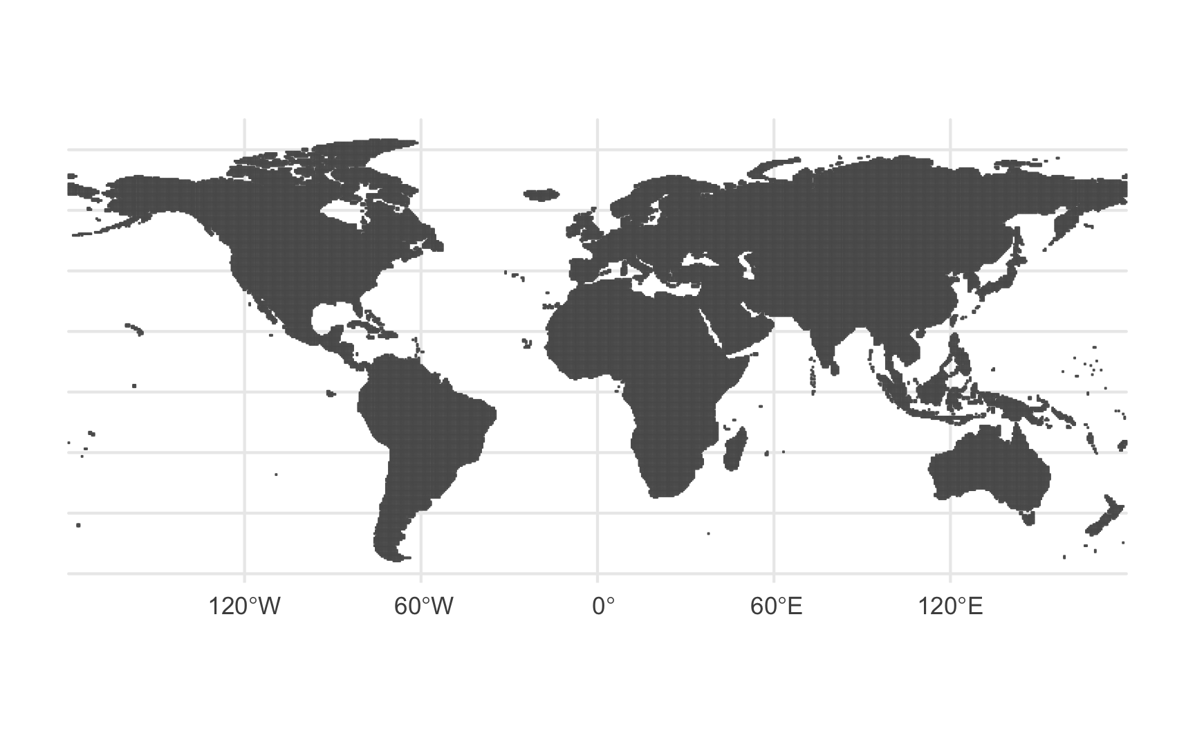
A specific country, Ethiopia, with cells filled by population:
clean_grid |>
  filter(country == "Ethiopia") |>
  ggplot(aes(fill = pop_gpw_sum)) +
  geom_sf() +
  scale_fill_viridis_c(option = "inferno",
                       end = .9,
                       trans = "log10",
                       labels = scales::comma,
                       name = "") +
  labs(title = "GRID-level population in Ethiopia")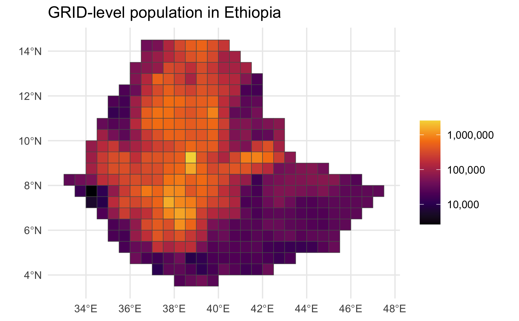
Log-transforming population is sometimes useful in maps, otherwise “outlier” units will swamp everything else, as with Addis Ababa below:
clean_grid |>
  filter(country == "Ethiopia") |>
  ggplot(aes(fill = pop_gpw_sum)) +
  geom_sf() +
  scale_fill_viridis_c(option = "inferno",
                       end = .9,
                       labels = scales::comma,
                       name = "") +
  labs(title = "GRID-level population in Ethiopia")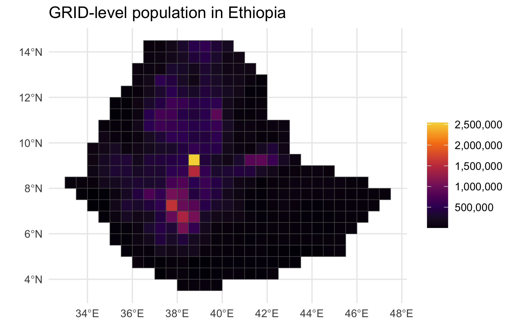
Finding neighbors
Doing most forms of spatial analysis requires knowing how the different units in the data relate to one another. With spatial data, it’s common to look at whether two units are neighbors or not. Being a neighbor might be defined as sharing a common border, the distances between the capitals, or centroids, or… whatever.
Let’s do this for just the United States, Mexico, and Canada:
three_countries =
  clean_grid |>
  filter(country %in% c("United States", "Mexico", "Canada"))

ggplot(three_countries, aes(fill = country)) + geom_sf()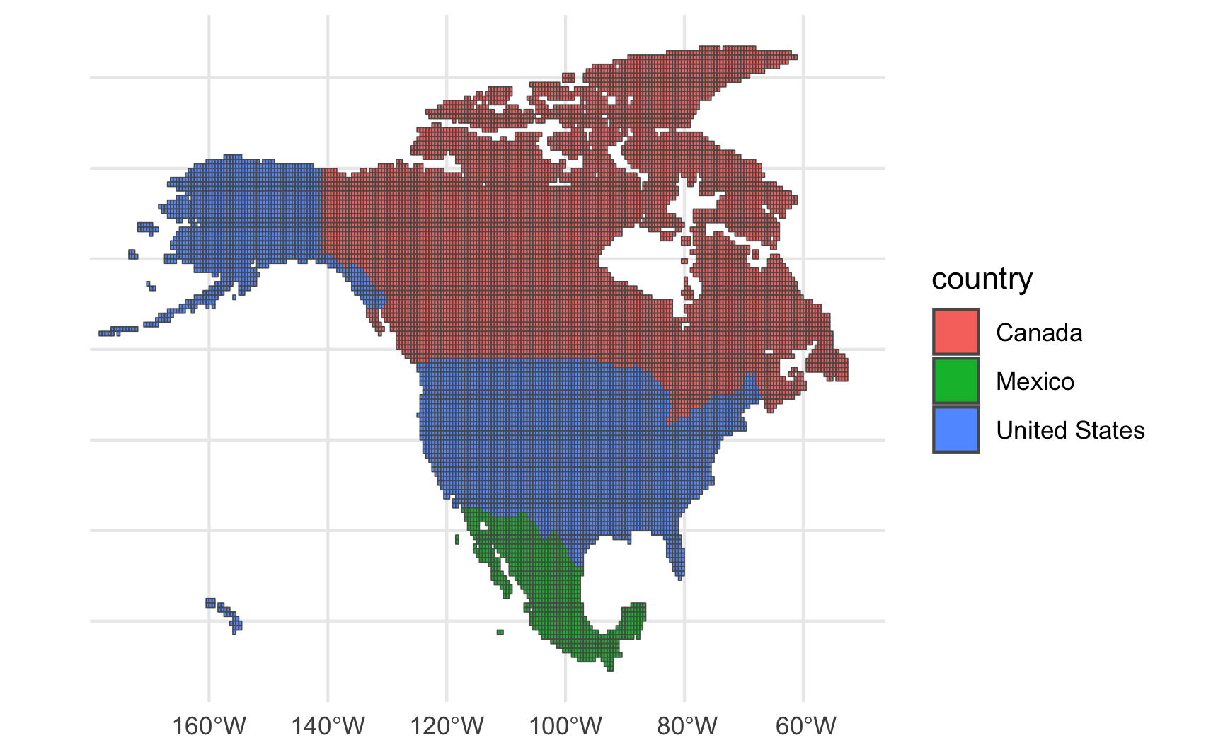
To describe these relationships, we use an N by N adjacency matrix, where N is the number of units in our data and any entry (i,j) tells us whether units i and j are neighbors or not.
To do this in R, I find the easiest thing is (unfortunately) to switch from sf to spdep package and use the spdep::poly2nb() function.
# convert back to sp object to use nice sp dep functions
three_countries_sp = as(three_countries, Class = "Spatial")
Below, we specify queen == FALSE because we want to use Rook’s contiguity (as opposed to Queen’s).
# get neighbors
nb = spdep::poly2nb(three_countries_sp,
             queen = FALSE,
             row.names = three_countries_sp$gid)
The output of our nb object looks like this, and tells us a bunch of information about what neighborhood relations among our units looks like, including whether any units were found to have no neighbors:
nb
## Neighbour list object:
## Number of regions: 13719
## Number of nonzero links: 52574
## Percentage nonzero weights: 0.02793
## Average number of links: 3.832
## 2 regions with no links:
## 211700 209569
## 19 disjoint connected subgraphs
So, for example, gid = 211700 has no neighbors.
Something prudent at this point would be to check whether the neighborhood list we got actually makes sense.
First, let’s look at a place that the nb object tells us has no neighbors, such as gid = 211700:
# plot place with no neighbors, Alaskan island
three_countries %>%
  filter(country == "Canada") %>%
  ggplot() +
  geom_sf() +
  # add the place with no neighbors (gid == 211700)
  geom_sf(data = filter(three_countries, gid == 211700), fill = "red") +
  # zoom in on location
  coord_sf(xlim = c(-180, -140), ylim = c(50, 70), expand = FALSE)
Checks out: looks like some tiny island that shouldn’t have neighbors.
Now, how about a place that should have neighbors? Let’s look at a random cell in Canada:
# plot place and its neighbors (in canada) # CHECKS OUT!
three_countries %>%
  filter(country == "Canada") %>%
  ggplot() + geom_sf() +
  # random place in canada
  geom_sf(data = filter(three_countries, gid == 249328), fill = "red") +
  # neighbors from nb object
  geom_sf(data = filter(three_countries, gid %in% c(249329,249327, 248608)), fill = "blue") +
  # zoom in on location
  coord_sf(xlim = c(-100, -50), ylim = c(75, 85), expand = FALSE)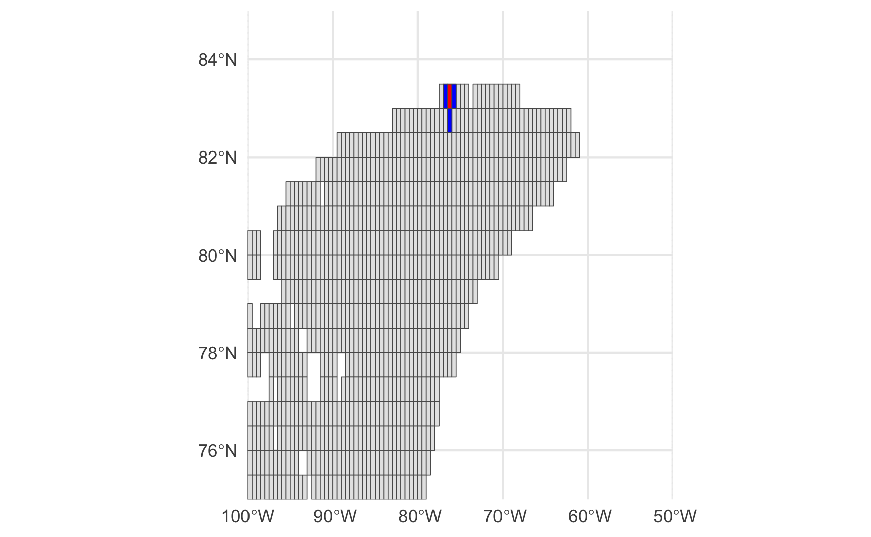
A bit hard to make out, but if you zoom in you will see that the nb object correctly identified this GRID’s neighbors.