What do controls do?

Introduction

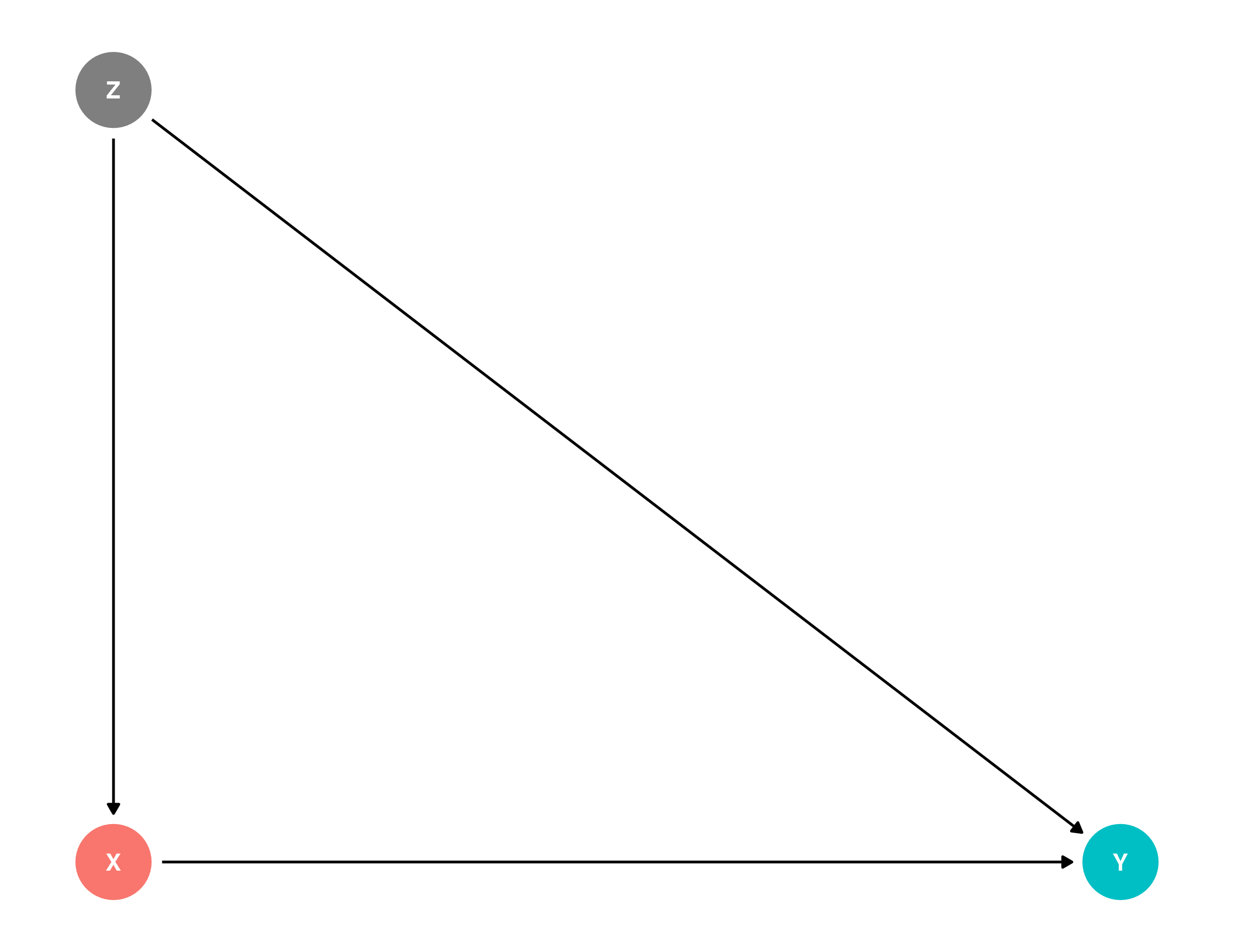
When I first learned about regression I found the use of controls mysterious. The “why” was clear: we have a situation where we want to estimate the effect of \(X\) on \(Y\), but there is a third variable, \(Z\), that affects both \(X\) and \(Y\). \(Z\) will confound our estimates of \(X\) on \(Y\), so we need to “control for” \(Z\) in our regression.

But what does it mean to “control” for Z? What does that “do”?

Some textbooks discuss controlling in terms of comparisons. Here’s Gelman in Regression and other stories:

We interpret the regression slopes as comparisons of individuals that differ in one predictor while being at the same levels of the other predictors.

Or from Nick Huntington-Klein’s The Effect:

If two observations have the same values of the other variables in the model, but one has a value of𝑋 that is one unit higher, the observation with the X one unit higher will on average have a𝑌that is B1 units higher

I love this intuition. We’d say that comparing two people of identical Z, we’d expect someone with an additional unit of \(X\) to have \(\beta_1\) more in \(Y\).

But how is regression doing this? What about the regression makes this comparison possible?

Here is one way of thinking about this that clarified regression controls for me and their limitations.

Example: ideology and campaign finance

Say we’re looking at Adam Bonica’s data on campaign finance, from my juanr package. Each row is a political candidate:

Sample of Bonica's campaign finance data

cycle	name	party	dwnom1	state	district	seat	incumbent	gender	num_distinct_donors	total_receipts	contribs_from_candidate	total_disbursements
2018	Van Risseghem, Anthony L	R	NA	WY	WYS18	senate	challenger	M	NA	0	0	0
2018	Holtz, John	R	NA	WY	WYS18	senate	challenger	M	NA	0	0	0
2018	Hardy, Charles E	R	NA	WY	WYS18	senate	challenger	M	39	8633	1843	8475
2018	De La Fuente, Roque Rocky	D	NA	WY	WYS18	senate	challenger	M	NA	0	0	0
2018	Miller, Rod	R	NA	WY	WY01	house	challenger	M	NA	0	0	0
2018	Stanley, Blake	R	NA	WY	WY01	house	challenger	M	NA	5820	4250	4314

Say we wanted to estimate the effect of ideology (dwnom1) on the amount of money raised (total_receipts). dwnom1 measures ideology using the DW-NOMINATE score, which theoretically ranges from -1 (left-wing) to 1 (right-wing).

We estimate a simple model, below. For the purposes of this exercise, let’s ignore the standard error and focus only on the point estimate.

	No controls
+ p < 0.1, * p < 0.05, ** p < 0.01, *** p < 0.001
(Intercept)	2418569.034***
	(105407.946)
dwnom1	-258416.541
	(225672.845)
Num.Obs.	1670

We see that more left-wing candidates tend to raise more money: going from a perfect moderate to a perfect left-winger results in a $258,416 increase in fundraising. Considering the median candidate raises about 15k, this is sizable.

Many things might confound this relationship. One potential confound (\(Z\)) is political party: the parties have different ideologies and might also have different fundraising capacities. So we control for party:

	No controls	Control for party
+ p < 0.1, * p < 0.05, ** p < 0.01, *** p < 0.001
(Intercept)	2418569.034***	3177880.673***
	(105407.946)	(364378.861)
dwnom1	-258416.541	1469866.143+
	(225672.845)	(814742.914)
partyI		-3325724.986***
		(457391.359)
partyR		-1653810.976*
		(727629.657)
Num.Obs.	1670	1670

Now the story is completely different: controlling for party, we see that more left-wing candidates raise less money. Going from a perfect moderate to a perfect left-winger results in almost 1.5 million less in fundraising.

Using the “comparisons” language from the textbooks, we can say that comparing two candidates from the same party, the more left-wing candidate raises less money.

But how do we get here?

Stratification

One way to think about the “comparisons” interpretation of controls is as a kind of stratification: when we control for \(Z\), what we would like to do is see if the relationship between \(X\) and \(Y\) “holds” within levels of \(Z\).

To put it in the “defensive” terms in which researchers typically operate: if someone says that the relationship between \(X\) and \(Y\) is confounded by \(Z\), the researcher can respond by looking at two people with the same value of \(Z\). If there is still a relationship between \(X\) and \(Y\), then \(Z\) alone doesn’t explain it away.

In our case, this would look like estimating the relationship between ideology and fundraising within each of the three parties in the data (Democrats, Republicans, and Independents):

bonica |>
  group_by(party) |>
  summarise(
    mod = list(lm_robust(total_receipts ~ dwnom1, data = cur_data()))
  ) |>
  mutate(tidy_mod = map(mod, broom::tidy)) |>
  unnest(tidy_mod) |>
  filter(term == "dwnom1") |>
  select(party, estimate, std.error, p.value) |>
  my_kbl(caption = "Effect of ideology on fundraising, by party")

Effect of ideology on fundraising, by party

party	estimate	std.error	p.value
D	5705276	2140241	0.01
I	52320	11542	0.00
R	-517739	714436	0.47

We see that within each party, the relationship between ideology and fundraising is different: large and positive for Democrats, larege and negative for Republicans, and weakly positive for Independents.

So how do we get from these three estimates to one overall estimate that controls for party, as in the model at the top of the page?

The answer is that regression is doing a kind of weighted average of these within-group estimates.

The weighting formula

When we estimate lm(Y ~ X + Z) where \(Z\) is categorical, the coefficient on \(X\) is a weighted average of the within-group slopes:

\[ \hat{\beta}_{\text{pooled}} = \frac{\sum_{g=1}^{G} w_g \cdot \hat{\beta}_g}{\sum_{g=1}^{G} w_g} \]

where \(\hat{\beta}_g\) is the slope of \(X\) on \(Y\) estimated within group \(g\), and the weight \(w_g\) is:

\[ w_g = (n_g - 1) \cdot \text{Var}_g(X) \]

That is, the weight for each group reflects two things:

1. Group size: groups with more observations contribute more squared deviations, so they get more weight. This makes sense — we have more information about the relationship in larger groups.
2. Within-group variance of \(X\): groups where the treatment variable \(X\) varies more get more weight. This also makes sense — if everyone in a group has the same value of \(X\), we can’t learn anything about the effect of \(X\) from that group.

This is an important result. It tells us that when we “control for \(Z\)”, we are not giving equal weight to every level of \(Z\). We are letting the levels of \(Z\) that have more data and more variation in \(X\) drive the overall estimate.

Checking this with the Bonica data

Let’s verify this with our running example. First, we compute the within-party slopes, group sizes, and variances of ideology:

# drop rows with missing ideology or receipts (same as lm does internally)
bonica_complete <- bonica |>
  filter(!is.na(dwnom1), !is.na(total_receipts))

# within-party estimates, sample sizes, and variance of X
strat <- bonica_complete |>
  group_by(party) |>
  summarise(
    beta_g = coef(lm(total_receipts ~ dwnom1))["dwnom1"],
    n_g = n(),
    var_g = var(dwnom1)
  ) |>
  mutate(
    weight = (n_g - 1) * var_g
  )

strat |>
  my_kbl(caption = "Within-party estimates and weights")

Within-party estimates and weights

party	beta_g	n_g	var_g	weight
D	5705276	770	0.02	12.07
I	52320	9	0.06	0.48
R	-517739	891	0.03	25.38

Now we can compute the weighted average and compare it to the OLS estimate:

# weighted average of within-party slopes
beta_weighted <- with(strat, sum(weight * beta_g) / sum(weight))

# OLS with party control
beta_ols <- coef(lm(total_receipts ~ dwnom1 + party, data = bonica_complete))["dwnom1"]

tibble(
  `Weighted average` = beta_weighted,
  `OLS with controls` = beta_ols
) |>
  my_kbl(caption = "Stratified weighted average vs. OLS coefficient")

Stratified weighted average vs. OLS coefficient

Weighted average	OLS with controls
1469866	1469866

The two estimates are the same.¹ This confirms that “controlling for party” in OLS is equivalent to: (1) estimating the ideology-fundraising relationship separately within each party, and (2) taking a weighted average of those estimates, where groups with more observations and more ideological variation get more influence.

¹ There can be minor numerical differences due to floating point arithmetic, but they are substantively identical.

What this tells us about controls

This decomposition clarifies a few things about what controls do and don’t do:

1. Controls are about within-group comparisons. When we control for \(Z\), we are comparing units that share the same value of \(Z\). The regression coefficient is a summary of these within-group relationships.

2. The summary is not a simple average. Groups with more data and more variation in \(X\) contribute more. This means the controlled estimate might be driven by a subset of the data that you didn’t intend to emphasize.

3. With categorical controls, the logic is transparent. We can literally split the data, estimate within each group, and see how the pieces combine.

4. With continuous controls, we’re trusting linearity. When \(Z\) is continuous, we can’t literally stratify — there are too many unique values of \(Z\). Instead, regression assumes the relationship between \(Z\) and \(Y\) is linear. This is a stronger assumption than the categorical case, where we make no assumptions about the shape of the \(Z\)-\(Y\) relationship within each group. If the true relationship between \(Z\) and \(Y\) is nonlinear, a linear control for \(Z\) may not fully “remove” the confounding.

The residuals approach: Frisch-Waugh-Lovell

There is a second way of thinking about what controls do that complements the stratification approach. Instead of asking “what is the relationship between \(X\) and \(Y\) within levels of \(Z\)?”, we can ask: “what is the relationship between the parts of \(X\) and \(Y\) that can’t be explained by \(Z\)?”

This is the idea behind the Frisch-Waugh-Lovell (FWL) theorem. The theorem says that the coefficient on \(X\) in lm(Y ~ X + Z) is identical to the coefficient you get from the following three-step procedure:

1. Regress \(Y\) on \(Z\) and save the residuals. Call these \(\tilde{Y}\). These are the parts of \(Y\) that \(Z\) can’t explain.
2. Regress \(X\) on \(Z\) and save the residuals. Call these \(\tilde{X}\). These are the parts of \(X\) that \(Z\) can’t explain.
3. Regress \(\tilde{Y}\) on \(\tilde{X}\).

The coefficient from step 3 is the same as the coefficient on \(X\) from the full model.

The intuition is straightforward: if \(Z\) confounds the relationship between \(X\) and \(Y\), we can remove its influence by stripping out everything \(Z\) explains from both variables. What’s left over — the residuals — are the “pure” variation in \(X\) and \(Y\), free of \(Z\). The relationship between those residuals is the controlled estimate.

Checking FWL with the Bonica data

Let’s verify this with our running example. We regress fundraising on party, save the residuals. Regress ideology on party, save the residuals. Then regress one on the other:

# step 1: residualize Y (fundraising) on Z (party)
resid_y <- residuals(lm(total_receipts ~ party, data = bonica_complete))

# step 2: residualize X (ideology) on Z (party)
resid_x <- residuals(lm(dwnom1 ~ party, data = bonica_complete))

# step 3: regress residualized Y on residualized X
beta_fwl <- coef(lm(resid_y ~ resid_x))["resid_x"]

tibble(
  `OLS with controls` = beta_ols,
  `Stratification (weighted avg)` = beta_weighted,
  `FWL (residuals)` = beta_fwl
) |>
  my_kbl(caption = "Three equivalent ways to get the controlled estimate")

Three equivalent ways to get the controlled estimate

OLS with controls	Stratification (weighted avg)	FWL (residuals)
1469866	1469866	1469866

All three approaches produce the same coefficient.

Because party is categorical, the residuals here have a nice interpretation: they are just the group-demeaned values. The residual of a Democrat’s ideology score is how far their ideology is from the average Democrat’s ideology. The residual of their fundraising is how much they raised relative to the average Democrat. In other words: among candidates who are more ideologically extreme for their party, do they raise more or less for their party?

Two intuitions for controls

We’ve now seen two equivalent ways of thinking about what regression controls do:

1. Stratification: split the data by \(Z\), estimate the \(X\)-\(Y\) relationship within each group, and take a weighted average. Controls ask: within levels of Z, is there still a relationship between X and Y?

2. Residualization (FWL): strip out what \(Z\) explains from both \(X\) and \(Y\), and look at what’s left. Controls ask: using only the variation in X and Y that Z can’t account for, is there a relationship?