Multicollinearity is a reality problem

causality

Author

Juan Tellez

Published

February 21, 2026

Introduction

In grad school I was introduced to the problem of “multicollinearity”. This is the idea that if your explanatory variables are “too” correlated this will create issues with the inferences you draw from the model. The way it’s presented is typically as a diagnostic problem. You use a diagnostic tool (e.g., a VIF statistic) and if the problem is “too” severe you are in trouble. At that point, some textbooks seem to endorse dropping variables or combining them via PCA.

But this hangs weirdly with the way we teach and think about causal inference. If I want to estimate a treatment effect, the other explanatory variables in my model should be there for a reason: I believe that they are confounds, and if I fail to adjust for them, I will reach the wrong conclusions about what I’m estimating. What if a multicollinearity diagnostic tells me to drop an important control?

Wooldridge pushes back on this in Introductory Econometrics. He argues that multicollinearity is not a violation of any OLS assumption and that textbooks which “test” for it or try to “solve” it are misleading. As he puts it, multicollinearity is essentially a variation problem: it means you don’t have enough variation in your data to precisely estimate what you want to estimate. Blanchard makes the point even more bluntly: “multicollinearity is God’s will, not a problem with OLS.”

This post uses a simulation to build intuition for what multicollinearity actually is and why Wooldridge and Blanchard are right.

Perfect collinearity: the easy case

Say we want to estimate the effect of press freedom on corruption. The idea is that media scrutiny deters corrupt behavior: countries with freer presses tend to have less corruption. We believe that regime type — whether a country is a democracy or not — confounds this relationship: democracies tend to have freer presses and tend to have less corruption. So we control for democracy.

Before we get to the interesting case, it’s worth being clear about the boring one. Perfect collinearity — where one regressor is an exact linear function of another — means the model literally cannot be estimated.

Imagine, in this case, that press freedom is a perfect function of regime type: every democracy gets a press freedom score of 1 and every autocracy gets a 0:

set.seed(123)
n <- 200
democracy <- rbinom(n, 1, 0.4)
press_freedom_perfect <- democracy
corruption_perfect <- -2 * press_freedom_perfect + rnorm(n)

lm(corruption_perfect ~ press_freedom_perfect + democracy) |>
  summary() |>
  coef()
##                       Estimate Std. Error  t value  Pr(>|t|)
## (Intercept)            0.06653    0.08713   0.7637 4.460e-01
## press_freedom_perfect -2.15404    0.13951 -15.4397 8.043e-36

R drops one of the terms. The reason is straightforward: if you know whether a country is a democracy, you know its press freedom score exactly. There is no observation in the data — and no observation that could exist — where press freedom changes but democracy doesn’t. So there is no way to estimate the independent effect of one holding the other constant.

This is a real constraint, but it’s also obvious. In practice, perfect collinearity comes up with things like including a full set of dummy variables alongside an intercept, or including a variable and its exact linear transformation.

The case that textbooks worry about — and that Wooldridge argues they worry about too much — is imperfect collinearity: when regressors are correlated but not perfectly so. In reality, press freedom is not a perfect function of democracy. Some autocracies have more press freedom than others; some democracies restrict theirs. There is variation within regime type — just not very much. This is the common scenario in applied work.

So let’s make the example realistic. The true effect of press freedom on corruption is \(\beta = -0.5\): for each unit increase in press freedom, corruption decreases by half a unit. Democracy independently boosts press freedom and reduces corruption. But now press freedom is continuous and only correlated with democracy, not determined by it:

set.seed(42)
n <- 200

# democracy is binary
democracy <- rbinom(n, 1, 0.4)

# press freedom: democracies have higher and more variable press freedom
press_freedom <- case_when(
  democracy == 1 ~ rnorm(n, mean = 7, sd = 1.5),
  democracy == 0 ~ rnorm(n, mean = 2, sd = 0.5)
)

# corruption: function of press freedom + democracy + noise
beta_true <- -0.5
corruption <- beta_true * press_freedom - 3 * democracy + rnorm(n, sd = 2)

df <- tibble(democracy = factor(democracy, labels = c("Autocracy", "Democracy")),
             press_freedom, corruption)

Here’s what the data looks like:

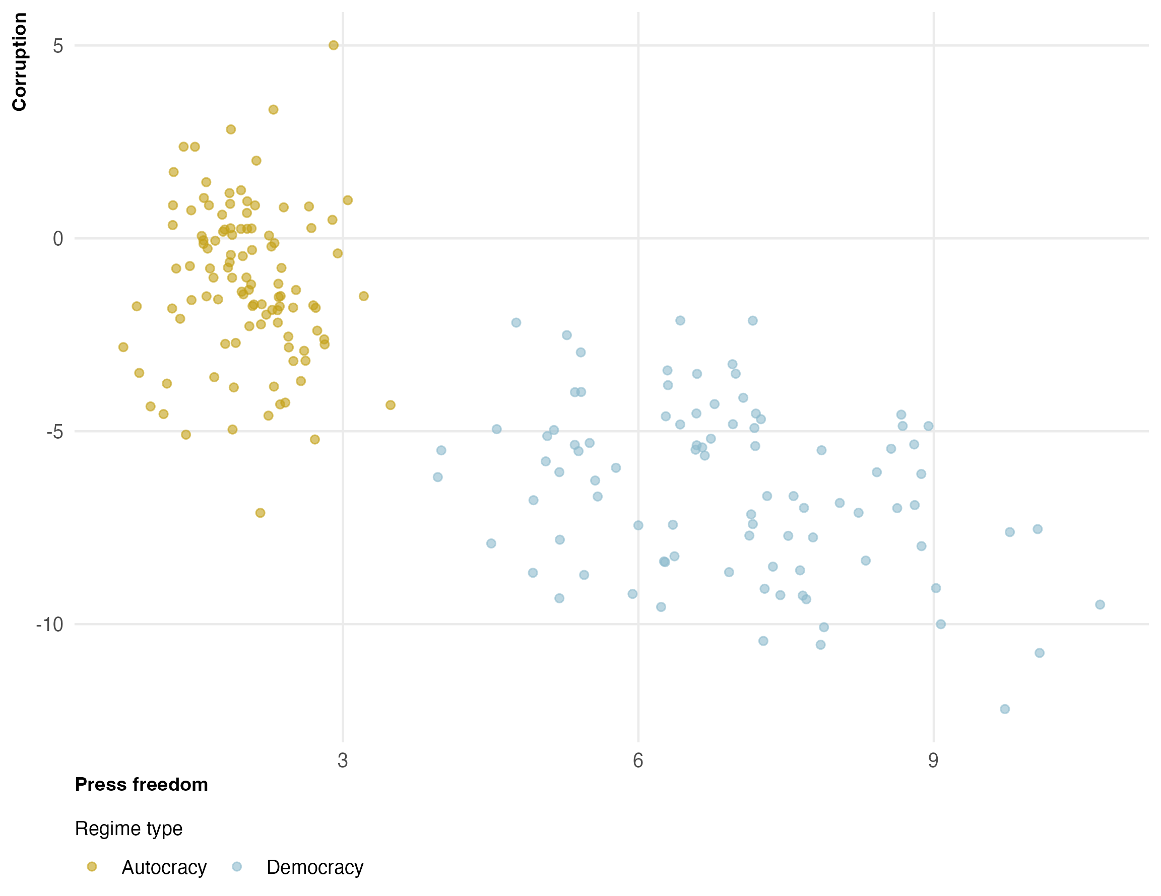
Two things are clear. First, there is a strong negative relationship between press freedom and corruption. Second, democracies and autocracies occupy very different regions of the press freedom axis. Within autocracies, press freedom barely varies — it’s almost always between 1 and 3.

This is the “multicollinearity”: press freedom and democracy are highly correlated, so when we control for democracy, there isn’t much variation left in press freedom to work with — especially within the autocracy group.

The naive and controlled estimates

library(estimatr)
library(modelsummary)

mod_naive <- lm_robust(corruption ~ press_freedom, data = df)
mod_controlled <- lm_robust(corruption ~ press_freedom + democracy, data = df)

modelsummary(list("No controls" = mod_naive,
                  "Control for democracy" = mod_controlled),
             gof_map = "nobs", stars = TRUE)

	No controls	Control for democracy
+ p < 0.1, * p < 0.05, p < 0.01, * p < 0.001
(Intercept)	0.676*	-0.136
	(0.277)	(0.338)
press_freedom	-1.000***	-0.494***
	(0.055)	(0.137)
democracyDemocracy		-2.946***
		(0.730)
Num.Obs.	200	200

The naive estimate overstates the effect of press freedom because it’s picking up the effect of democracy. The controlled estimate is closer to the truth (\(\beta = -0.5\)) — but the standard error is much larger. This is multicollinearity at work.

What’s happening: the stratification view

As we saw in the controls post, controlling for democracy is equivalent to estimating the press freedom-corruption relationship within each regime type and taking a weighted average. The plot below makes the problem visible:

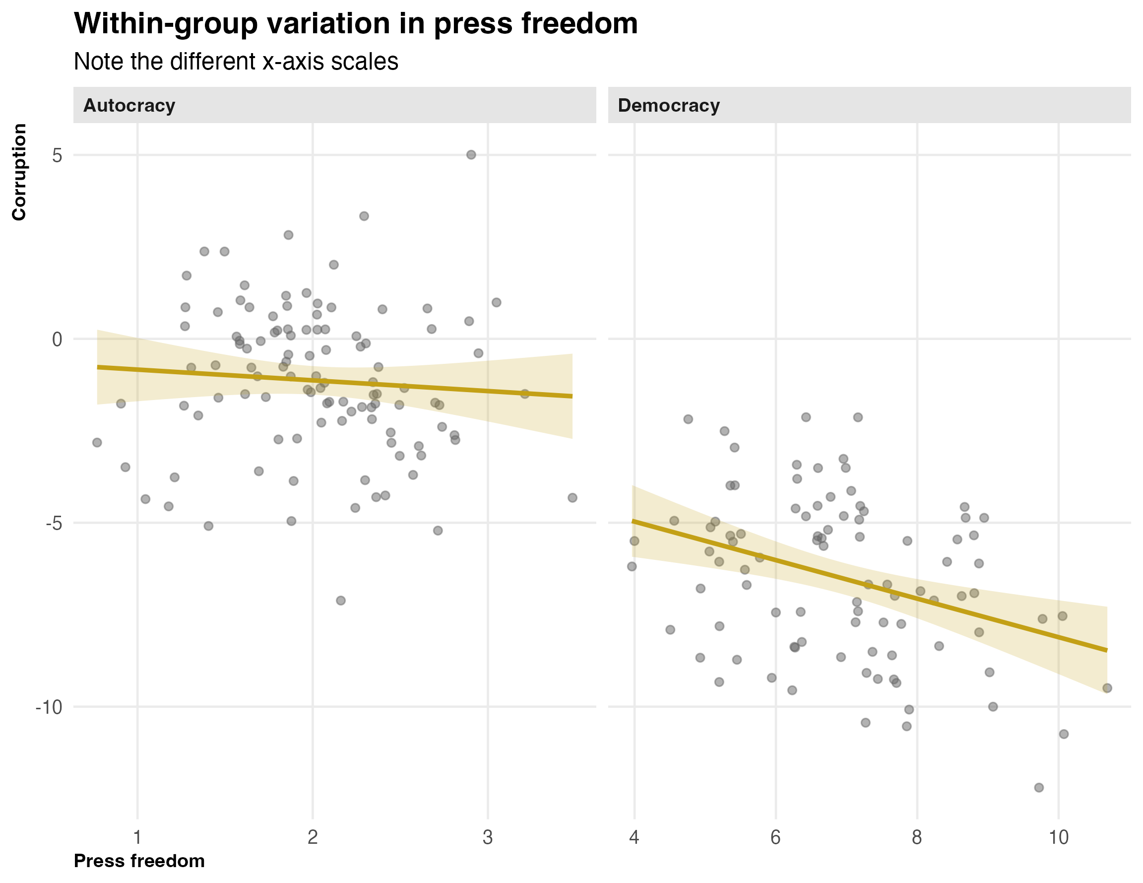
Look at the x-axes. Among democracies, press freedom ranges from about 3 to 11 — plenty of variation to estimate a slope. Among autocracies, it’s crammed between about 1 and 3. The regression line is there, but the confidence band is enormous because there’s almost nothing to work with. The overall controlled estimate is being driven almost entirely by the democracy subsample.

This is the Wooldridge point. The “problem” isn’t that the regression is doing something wrong. OLS is unbiased. The problem is that the data doesn’t give us enough within-group variation to estimate the effect precisely. That’s a property of the world — autocracies really do have uniformly low press freedom — not a flaw in the method.

Simulation: imprecision, not bias

To make this concrete, let’s run the same data-generating process many times and look at the sampling distribution of the controlled estimate:

simulate_once <- function(n = 200) {
  democracy <- rbinom(n, 1, 0.4)
  press_freedom <- case_when(
    democracy == 1 ~ rnorm(n, mean = 7, sd = 1.5),
    democracy == 0 ~ rnorm(n, mean = 2, sd = 0.5)
  )
  corruption <- -0.5 * press_freedom - 3 * democracy + rnorm(n, sd = 2)
  d <- tibble(democracy, press_freedom, corruption)

  mod <- lm(corruption ~ press_freedom + democracy, data = d)
  coef(mod)["press_freedom"]
}

sims <- tibble(beta_hat = map_dbl(1:1000, ~simulate_once()))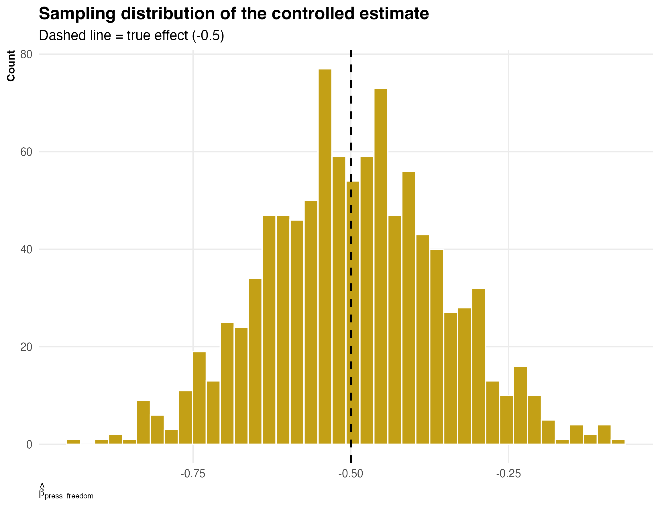

The distribution is centered on the truth. OLS is unbiased. But the distribution is wide — in any given sample, the estimate could be quite far from -0.5. This is what imprecision looks like.

The “cure” is worse than the disease

Now, what do some textbooks recommend? Drop the collinear variable. Let’s see what happens if we drop the democracy control:

sims_no_control <- tibble(
  beta_hat = map_dbl(1:1000, function(i) {
    democracy <- rbinom(200, 1, 0.4)
    press_freedom <- case_when(
      democracy == 1 ~ rnorm(200, mean = 7, sd = 1.5),
      democracy == 0 ~ rnorm(200, mean = 2, sd = 0.5)
    )
    corruption <- -0.5 * press_freedom - 3 * democracy + rnorm(200, sd = 2)
    coef(lm(corruption ~ press_freedom))["press_freedom"]
  })
)

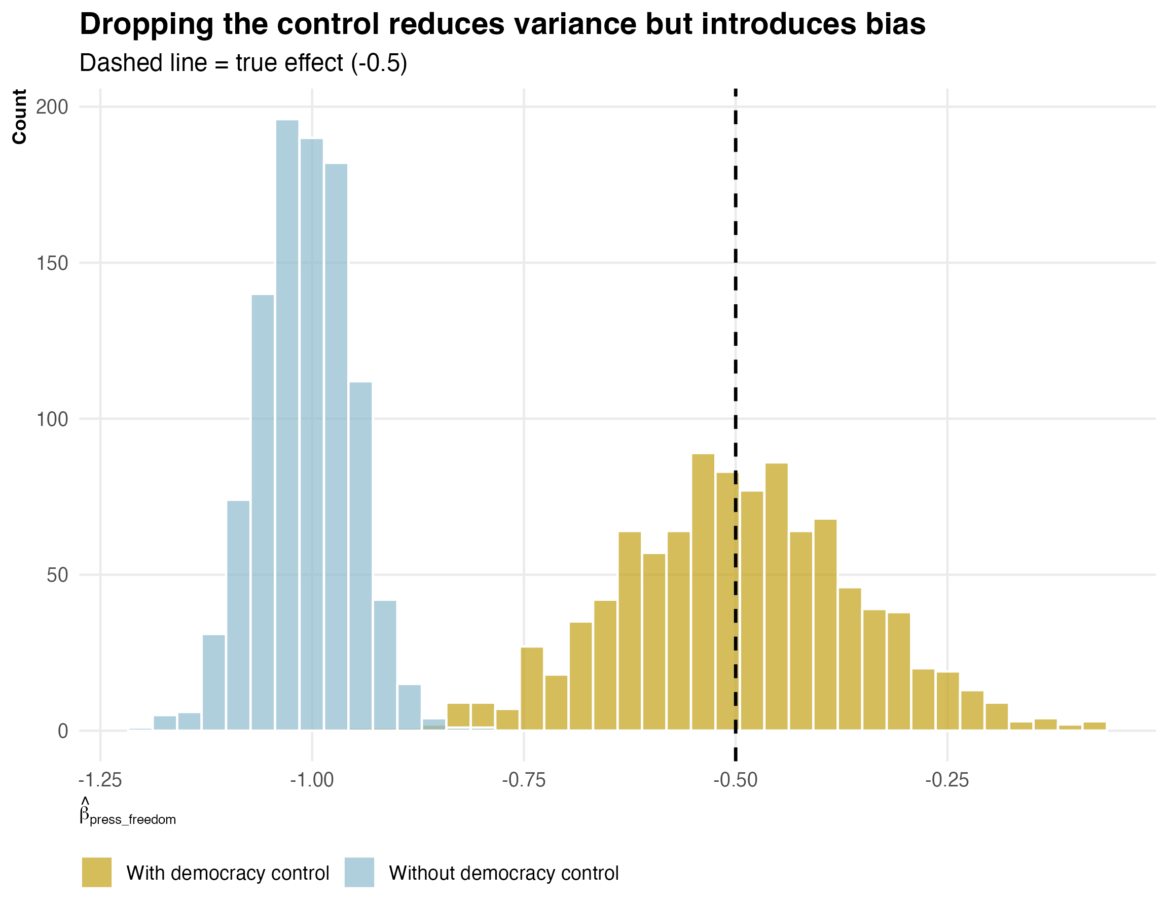
The uncontrolled estimates are more precise — the distribution is tighter. But they are biased: the distribution is centered well below -0.5 because the regression attributes some of democracy’s effect on corruption to press freedom.

This is why Wooldridge’s framing matters. If you think of multicollinearity as a disease with a “cure” (dropping variables), you are trading one problem (wide confidence intervals) for another (omitted variable bias).

Summary

Multicollinearity means your regressors are correlated. When you control for a variable that is highly correlated with your treatment, you’re left with little variation to estimate the treatment effect. Your estimates will be imprecise. This is annoying but it’s not a methodological failure. It’s the data telling you that it can’t cleanly distinguish the effects of two things that move together.